This year, we’re celebrating 10 years of Drive Stats. Coincidentally, we also made some upgrades to how we run our Drive Stats reports. We reported on how an attempt to migrate triggered a weeks-long recalculation of the dataset, leading us to map the architecture of the Drive Stats data.
This follow-up article focuses on the improvements we made after we fixed the existing bug (because hey, we were already in there), and then presents some of our ideas for future improvements. Remember that those are just ideas so far—they may not be live in a month (or ever?), but consider them good food for thought, and know that we’re paying attention so that we can pass this info along to the right people.
Now, onto the fun stuff.
Quick Refresh: Drive Stats Data Architecture
The podstats generator runs on every Storage Pod, what we call any host that holds customer data, every few minutes. It’s a C++ program that collects SMART stats and a few other attributes, then converts them into an .xml file (“podstats”). Those are then pushed to a central host in each datacenter and bundled. Once the data leaves these central hosts, it has entered the domain of what we will call Drive Stats.
Now let’s go into a little more detail: when you’re gathering stats about drives, you’re running a set of modules with dependencies to other modules, forming a data-dependency tree. Each time a module “runs”, it takes information, modifies it, and writes it to a disk. As you run each module, the data will be transformed sequentially. And, once a quarter, we run a special module that collects all the attributes for our Drive Stats reports, collecting data all the way down the tree.
Here’s a truncated diagram of the whole system, to give you an idea of what the logic looks like:
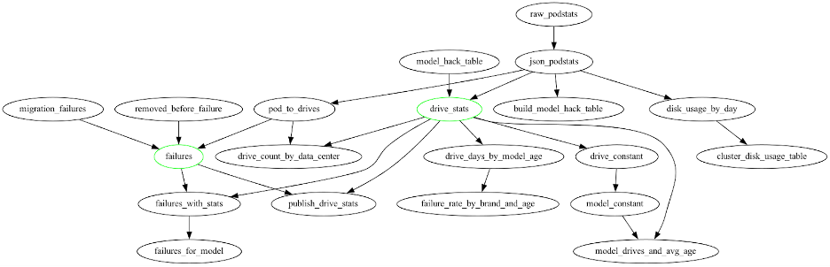
As you move down through the module layers, the logic gets more and more specialized. When you run a module, the first thing the module does is check in with the previous module to make sure the data exists and is current. It caches the data to disk at every step, and fills out the logic tree step by step. So for example, drive_stats, being a “per-day” module, will write out a file such as /data/drive_stats/2023-01-01.json.gz when it finishes processing. This lets future modules read that file to avoid repeating work.
This work deduplication process saves us a lot of time overall—but it also turned out to be the root cause of our weeks-long process when we were migrating Drive Stats to our new host. We fixed that by implementing versions to each module.
While You’re There… Why Not Upgrade?
Once the dust from the bug fix had settled, we moved forward to try to modernize Drive Stats in general. Our daily report still ran quite slowly, on the order of several hours, and there was some low-hanging fruit to chase.
Waiting On You, failures_with_stats
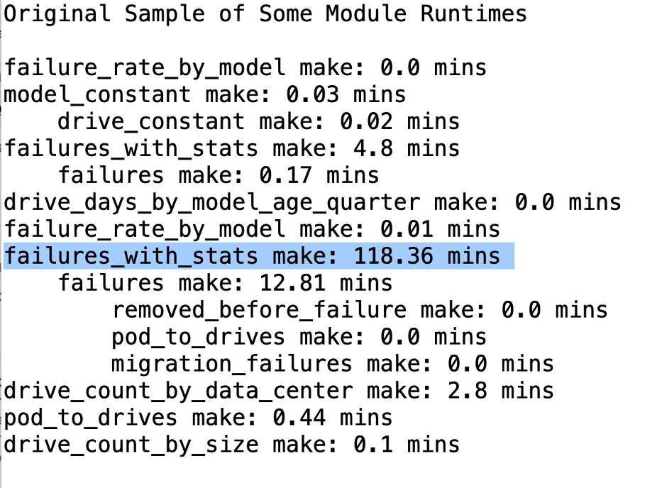
First things first, we saved a log of a run of our daily reports in Jenkins. Then we wrote an analyzer to see which modules were taking a lot of time. failures_with_stats was our biggest offender, running for about two hours, while every other module took about 15 minutes.
Upon investigation, the time cost had to do with how the date_range module works. This takes us back to caching: our module checks if the file has been written already, and if it has, it uses the cached file. However, a date range is written to a single file. That is, Drive Stats will recognize “Monday to Wednesday” as distinct from “Monday to Thursday” and re-calculate the entire range. This is a problem for a workload that is essentially doing work for all of time, every day.
On top of this, the raw Drive Stats data, which is a dependency for failures_with_stats, would be gzipped onto a disk. When each new query triggered a request to recalculate all-time data, each dependency would pick up the podstats file from disk, decompress it, read it into memory, and do that for every day of all time. We were picking up and processing our biggest files every day, and time continued to make that cost larger.
Our solution was what I called the “Date Range Accumulator.” It works as follows:
- If we have a date range like “all of time as of yesterday” (or any partial range with the same start), consider it as a starting point.
- Make sure that the version numbers don’t consider our starting point to be too old.
- Do the processing of today’s data on top of our starting point to create “all of time as of today.”
To do this, we read the directory of the date range accumulator, find the “latest” valid one, and use that to determine the delta (change) to our current date. Basically, the module says: “The last time I ran this was on data from the beginning of time to Thursday. It’s now Friday. I need to run the process for Friday, and then add that to the compiled all-time.” And, before it does that, it double checks the version number to avoid errors. (As we noted in our previous article, if it doesn’t see the correct version number, instead of inefficiently running all data, it just tells you there is a version number discrepancy.)
The code is also a bit finicky—there are lots of snags when it comes to things like defining exceptions, such as if we took a drive out of the fleet, but it wasn’t a true failure. The module also needed to be processable day by day to be usable with this technique.
Still, even with all the tweaks, it’s massively better from a runtime perspective for eligible candidates. Here’s our new failures_with_stats runtime:
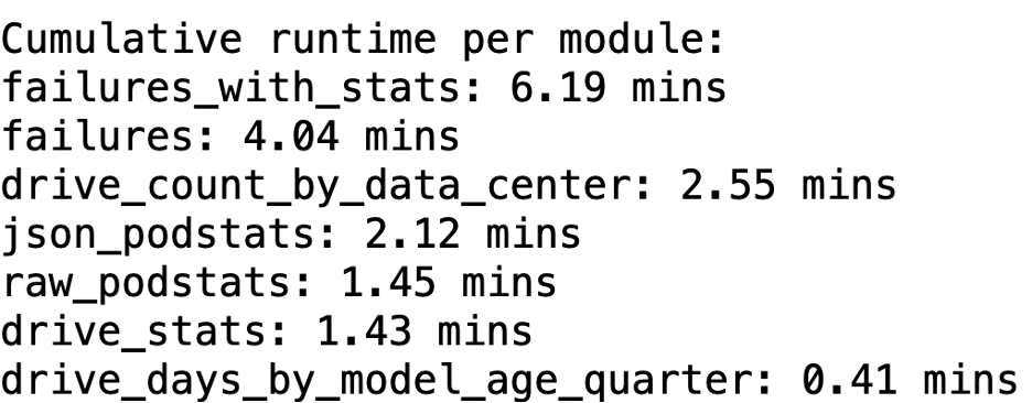
Note that in this example, we’re running that 60-day report. The daily report is quite a bit quicker. But, at least the 60-day report is a fixed amount of time (as compared with the all-time dataset, which is continually growing).
Code Upgrade to Python 3
Next, we converted our code to Python 3. (Shout out to our intern, Anath, who did amazing work on this part of the project!) We didn’t make this improvement just to make it; no, we did this because I wanted faster JSON processors, and a lot of the more advanced ones did not work with Python 2. When we looked at the time each module took to process, most of that was spent serializing and deserializing JSON.
What Is JSON Parsing?
JSON is an open standard file format that uses human readable text to store and transmit data objects. Many modern programming languages include code to generate and parse JSON-format data. Here’s how you might describe a person named John, aged 30, from New York using JSON:
{
“firstName”: “John”,
“age”: 30,
“State”: “New York”
}
You can express those attributes into a single line of code and define them as a native object:
x = { 'name':'John', 'age':30, 'city':'New York'}
“Parsing” is the process by which you take the JSON data and make it into an object that you can plug into another programming language. You’d write your script (program) in Python, it would parse (interpret) the JSON data, and then give you an answer. This is what that would look like:
import json

# some JSON:
x = '''
{
	"firstName": "John",
	"age": 30,
	"State": "New York"
}
'''

# parse x:
y = json.loads(x)

# the result is a Python object:
print(y["name"])
If you run this script, you’ll get the output “John.” If you change print(y["name"]) to print(y["age"]), you’ll get the output “30.” Check out this website if you want to interact with the code for yourself. In practice, the JSON would be read from a database, or a web API, or a file on disk rather than defined as a “string” (or text) in the Python code. If you are converting a lot of this JSON, small improvements in efficiency can make a big difference in how a program performs.
And Implementing UltraJSON
Upgrading to Python 3 meant we could use UltraJSON. This was approximately 50% faster than the built-in Python JSON library we used previously.
We also looked at the XML parsing for the podstats files, since XML parsing is often a slow process. In this case, we actually found our existing tool is pretty fast (and since we wrote it 10 years ago, that’s pretty cool). Off-the-shelf XML parsers take quite a bit longer because they care about a lot of things we don’t have to: our tool is customized for our Drive Stats needs. It’s a well known adage that you should not parse XML with regular expressions, but if your files are, well, very regular, it can save a lot of time.
What Does the Future Hold?
Now that we’re working with a significantly faster processing time for our Drive Stats dataset, we’ve got some ideas about upgrades in the future. Some of these are easier to achieve than others. Here’s a sneak peek of some potential additions and changes in the future.
Data on Data
In keeping with our data-nerd ways, I got curious about how much the Drive Stats dataset is growing and if the trend is linear. We made this graph, which shows the baseline rolling average, and has a trend line that attempts to predict linearly.
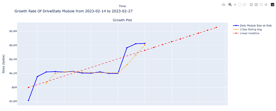
I envision this graph living somewhere on the Drive Stats page and being fully interactive. It’s just one graph, but this and similar tools available on our website would be 1) fun and 2) lead to some interesting insights for those who don’t dig in line by line.
What About Changing the Data Module?
The way our current module system works, everything gets processed in a tree approach, and they’re flat files. If we used something like SQLite or Parquet, we’d be able to process data in a more depth-first way, and that would mean that we could open a file for one module or data range, process everything, and not have to read the file again.
And, since one of the first things that our Drive Stats expert, Andy Klein, does with our .xml data is to convert it to SQLite, outputting it in a queryable form would save a lot of time.
We could also explore keeping the data as a less-smart filetype, but using something more compact than JSON, such as MessagePack.
Can We Improve Failure Tracking and Attribution?
One of the odd things about our Drive Stats datasets is that they don’t always and automatically agree with our internal data lake. Our Drive Stats outputs have some wonkiness that’s hard to replicate, and it’s mostly because of exceptions we build into the dataset. These exceptions aren’t when a drive fails, but rather when we’ve removed it from the fleet for some other reason, like if we were testing a drive or something along those lines. (You can see specific callouts in Drive Stats reports, if you’re interested.) It’s also where a lot of Andy’s manual work on Drive Stats data comes in each month: he’s often comparing the module’s output with data in our datacenter ticket tracker.
These tickets come from the awesome data techs working in our data centers. Each time a drive fails and they have to replace it, our techs add a reason for why it was removed from the fleet. While not all drive replacements are “failures”, adding a root cause to our Drive Stats dataset would give us more confidence in our failure reporting (and would save Andy comparing the two lists).
The Result: Faster Drive Stats and Future Fun
These two improvements (the date range accumulator and upgrading to Python 3) resulted in hours, and maybe even days, of work saved. Even from a troubleshooting point of view, we often wouldn’t know if the process was stuck, or if this was the normal amount of time the module should take to run. Now, if it takes more than about 15 minutes to run a report, you’re sure there’s a problem.
While the Drive Stats dataset can’t really be called “big data”, it provides a good, concrete example of scaling with your data. We’ve been collecting Drive Stats for just over 10 years now, and even though most of the code written way back when is inherently sound, small improvements that seem marginal become amplified as datasets grow.
Now that we’ve got better documentation of how everything works, it’s going to be easier to keep Drive Stats up-to-date with the best tools and run with future improvements. Let us know in the comments what you’d be interested in seeing.