Iceberg on Backblaze B2

If you work with cloud storage and data lakes, you’re likely hearing the word “Iceberg” with increasing frequency, occasionally prefixed by “Apache”. What is Apache Iceberg, and how can you leverage it to efficiently store data in object stores such as Backblaze B2 Cloud Storage? I’ll answer both of those questions in this blog post.

But, first, join me on a brief trip back in time to the beginning of the twenty-first century, a long-ago time before the emergence of big data and cloud computing.

CSV: The lingua franca of tabular data

In the early 2000s, if you were working with tabular data, you were likely using either a relational database management system (RDBMS), such as Oracle Database, or a spreadsheet, likely Microsoft Excel.

Data stored in an RDBMS is highly structured, meaning that it MUST conform to a predefined schema. For example, you might create an employee table with columns such as first name, last name, date of birth, hire date, and so on. The database schema holds metadata such as the name and data type of each column, whether that column must have a value, relationships between tables, and so on.

A spreadsheet, on the other hand, has some structure—data is arranged in rows and columns, similarly to an RDBMS–but each cell can contain anything: text, a number, a formula referencing other cells, even an image in today’s spreadsheets. We say that a spreadsheet is semi-structured data.

At the turn of the century, each database and spreadsheet had its own proprietary file format, optimized for its own requirements, and often not at all publicly documented, but the need to be able to exchange data between applications led to broad adoption of a file format to allow just that: comma-separated values, or CSV.

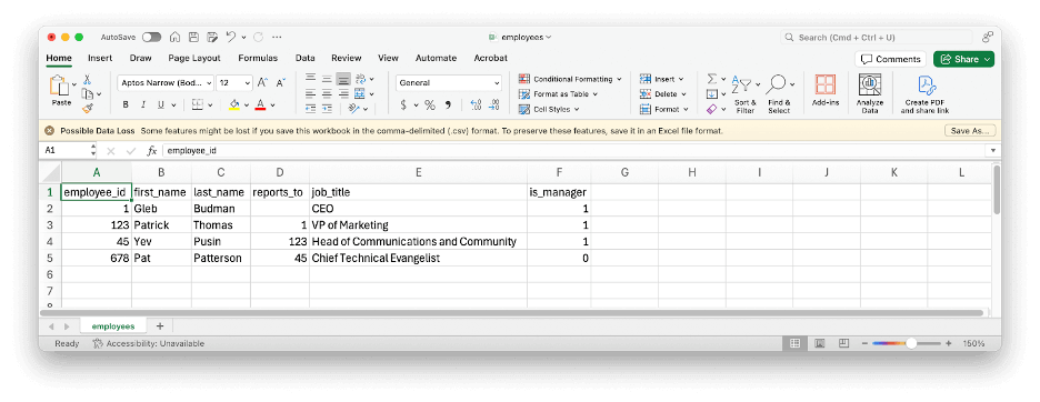
Here’s a simple example of some tabular data represented as CSV:

employee_id,first_name,last_name,reports_to,job_title,is_manager
1,Gleb,Budman,,CEO,1
123,Patrick,Thomas,1,"VP of Marketing",1
45,Yev,Pusin,123,"Head of Communications and Community",1
678,Pat,Patterson,45,"Chief Technical Evangelist",0

CSV is simple and flexible enough that it was easy for me to type that example up manually and import it into Microsoft Excel with no problems at all. Note that, as well as the commas, the double quotes in the CSV data are part of the file format, and do not appear in the imported data:

CSV has a lot of advantages: It’s simple; flexible; widely understood; the optional header line means that data can be somewhat self-describing; and it’s not controlled by any single vendor.

CSV does, however, also have a few disadvantages, including:

• There’s no schema; nothing in that file expresses that the values in the first column, apart from the header, must be integers.
• It’s difficult to represent complex or hierarchical datasets.
• Data is stored as text, which is inefficient for numerical and repetitive data. Text representations of numbers occupy more storage than binary, and applications must convert them to binary when loading the file and convert them back to text when saving it.

Avro, Parquet and ORC: File formats for big data

The emergence of open-source distributed computing frameworks such as Apache Hadoop and, later, Apache Spark, in the first two decades of this century drove the creation and adoption of more efficient ways of storing tabular data. Avro, Parquet and ORC, all Apache projects, are binary file formats that address shortcomings of CSV, such as encapsulating schema alongside the data.

Avro, like CSV, is designed for row-oriented data, which makes it well-suited to use cases that involve appending new data to files. Parquet and ORC, in contrast, are column-oriented file formats, perfect for online analytical processing (OLAP) use cases where, for example, an application might read an entire column from a table to calculate the sum of its values. As well as storing numbers in a binary representation, Parquet and ORC can also reduce file size through compression strategies such as run-length encoding.

Here’s a concrete example: The Drive Stats data set for December 2024 occupies 3.7GB of storage in CSV format. As Parquet, the same data consumes just 242MB, a data compression ratio of more than 15:1.

Why does it matter if your dataset is smaller? Well, beyond just cost savings, which are amplified when dealing with huge datasets, smaller files mean that running queries against full datasets takes less time, which reduces server load, compute costs, and so on.  

From file formats to table formats and data lakes

Apache Hadoop’s original use case was as an implementation of MapReduce, a programming model for manipulating large datasets. Engineers at Facebook, tasked with allowing SQL queries over datasets generated by Hadoop, created Apache Hive, and, with it, the Hive table format, which specified how to view a collection of files as a single logical table. The Hive table format in turn allowed organizations to create data lakes, repositories that store structured and semi-structured data in their original format for analysis by a wide range of tools, and, later, data lakehouses, which aim to combine the benefits of data lakes and traditional data warehouses by storing structured data using data lake tools and technologies.

A key concept of the Hive table format is partitioning, a way of organizing files to reduce the amount of data that must be read to process a query. Taking the Drive Stats dataset as an example, we can partition the files by year and month, so that each file has a prefix of the form:

/drivestats/year={year}/month={month}/

For example:

/drivestats/year=2024/month=12/

With this partitioning scheme, a system processing a query for hard drive statistics for, say, December 12, 2024, need only retrieve files with the above prefix. You might be wondering, “Why not partition the data on day, also, to further reduce the number of files that must be retrieved?” The answer depends on the data volume and access patterns. It’s much more efficient to partition data into fewer large files than many small files, so overly granular partitioning can actually impair performance.

It’s worth mentioning that file formats and table formats are largely independent of each other. You can use Avro, Parquet, ORC, or even CSV files with the Hive table format.

For more detail on the Parquet file format, Hive table format, and partitioning, see the blog post, Storing and Querying Analytical Data in Backblaze B2.

“Iceberg, captain, dead ahead!”

While the Hive table format served the big data community well for several years, it had a number of shortcomings:

• Every query incurs a file list (“list objects”, in S3 API terms) operation, which is particularly expensive with cloud object storage, both in terms of time and API transaction charges.
• Deleting or modifying data typically implies rewriting an entire data file, even if only a single row was affected.
• Hive can only partition datasets on columns that are in the table schema. For example, the Drive Stats data set includes a date column, so to use it with Hive, we had to create additional, redundant, year and month columns.
• Any changes to the data schema or partitioning strategy require affected files to be rewritten, making schema evolution problematic, if not infeasible, for large datasets.
• There is limited support for the kind of ACID (Atomic, Consistent, Isolated, Durable) transactions that are familiar from the RDBMS world. Attempts to add transaction support to Hive were not widely or consistently supported.

As a result, vendors and the broader big data community formed a number of projects to define new table formats to succeed Hive, including Apache Iceberg, Apache Hudi, and Delta Lake, a Linux Foundation project.

The three are broadly comparable in terms of features, but, over the past couple of years, Iceberg has emerged as the leader in terms of vendor adoption, with Snowflake announcing general availability of Iceberg tables in June 2024, and Amazon announcing S3 Tables, its managed Iceberg offering, in December 2024. Significantly, Databricks, the prime mover behind Delta Lake, acquired Tabular, a company founded by the original creators of Apache Iceberg, in June 2024, establishing its own beachhead in the Iceberg community.

Iceberg‘s features allow it to be used to organize huge data sets, efficiently and flexibly:

• Table metadata including the list of files that comprise a table is stored as JSON data alongside the data files, eliminating the need to run an expensive list object operation for every query.
• Schema evolution allows you to add, drop, update, or rename columns.
• Hidden partitioning decouples partitioning from the table schema. For example, you can partition data like the Drive Stats dataset by year and month based on the existing date values, without creating additional columns.
• Partition layout evolution allows you to modify your partitioning strategy as data volume or access patterns change.
• Time travel allows you to query table snapshots.
• Serializable isolation provides atomic table changes, ensuring readers never see inconsistent data.
• Multiple concurrent writers use optimistic concurrency, retrying to ensure that compatible updates succeed while detecting conflicting writes.

Iceberg is widely supported across the big data ecosystem, with many applications and tools  allowing you to store Iceberg tables in S3 compatible cloud object storage such as Backblaze B2. In this article, I’ll look at the simplest use case, running queries against the Drive Stats dataset, with three representative examples: Snowflake, Trino, and DuckDB.

Writing Iceberg data to Backblaze B2

I wrote a simple Python application, drivestats2iceberg, using the PyIceberg library, that converts the Drive Stats dataset from the zipped CSV files we publish to Parquet files in an Iceberg table stored in a Backblaze B2 Bucket. There are some useful techniques in drivestats2iceberg, and it is published on GitHub as open source, under the MIT license, so feel free to use it as a starting point for your own data conversion apps.

Querying Iceberg tables in Backblaze B2 from Snowflake

Snowflake is a data-as-a-service platform addressing a wide variety of use cases, including artificial intelligence (AI), machine learning (ML), collaboration across organizations, and data lakes.

As I mentioned above, Snowflake announced general availability of its Iceberg tables offering in June 2024, allowing you to manipulate Iceberg tables located on external volumes, outside your Snowflake warehouse, and query them alongside data in Snowflake-managed tables.

Snowflake’s Iceberg implementation is quite complicated, with different capabilities according to your choice of cloud object storage provider and whether you want Snowflake to manage your Iceberg catalog or use a catalog integration.

For our simple use case, where the Iceberg metadata and data files already exist in a Backblaze B2 Bucket, the first step is to create a Snowflake external volume, configuring it with suitable credentials and the location of the Drive Stats data.

Note: the application key shown in this Snowflake statement has read-only access to the drivestats-iceberg bucket. You can use it to query the Drive Stats data set from your own Snowflake instance or from other environments.

CREATE EXTERNAL VOLUME drivestats_b2
  STORAGE_LOCATIONS = (
    (
      NAME = 'b2_storage_location'
      STORAGE_PROVIDER = 'S3COMPAT'
      STORAGE_BASE_URL = 's3compat://drivestats-iceberg/'
      CREDENTIALS = (
        AWS_KEY_ID = '0045f0571db506a0000000017'
        AWS_SECRET_KEY = 'K004Fs/bgmTk5dgo6GAVm2Waj3Ka+TE'
      )
      STORAGE_ENDPOINT = 's3.us-west-004.backblazeb2.com'
    )
  )
  ALLOW_WRITES = FALSE;

Next, you must create a catalog integration. The object store catalog integration simply reads Iceberg metadata from an external (to Snowflake) cloud storage location:

CREATE CATALOG INTEGRATION my_iceberg_catalog_integration
  CATALOG_SOURCE = OBJECT_STORE
  TABLE_FORMAT = ICEBERG
  ENABLED = TRUE;

Now you can create an Iceberg table object that references the existing dataset. Note that Snowflake requires you to explicitly specify the metadata file to use for column definitions; this is typically the most recently created JSON file under the metadata prefix.

CREATE ICEBERG TABLE drivestats
  EXTERNAL_VOLUME = 'drivestats_b2'
  CATALOG = 'my_iceberg_catalog_integration'
  METADATA_FILE_PATH = 'drivestats/metadata/00225-317608b1-35a6-4135-8393-7543583623db.metadata.json';

That done, you can start querying the data:

How many records are in the current Drive Stats dataset?

SELECT COUNT(*) 
FROM drivestats;

Result:

564566016

How many hard drives was Backblaze spinning on a given date?

SELECT COUNT(*) 
FROM drivestats 
WHERE date = DATE '2024-12-31';

Result:

305180

How many exabytes of raw storage was Backblaze managing on a given date?

SELECT ROUND(SUM(CAST(capacity_bytes AS BIGINT))/1e+18, 2) 
FROM drivestats 
WHERE date = DATE '2024-12-31';

Result:

4.42

What are the top 10 most common drive models in the dataset?

SELECT model, COUNT(DISTINCT serial_number) AS count 
FROM drivestats 
GROUP BY model
ORDER BY count DESC
LIMIT 10;

Results (in drive days):

TOSHIBA MG08ACA16TA   40859
TOSHIBA MG07ACA14TA   39387
ST12000NM0007         38843
ST4000DM000           37040
ST16000NM001G         34501
WDC WUH722222ALE6L4   30148
WDC WUH721816ALE6L4   26547
ST12000NM0008         21028
HGST HMS5C4040BLE640  16349
ST8000NM0055          15680

My x-small Snowflake warehouse executed the first three queries in a fraction of a second. As you might expect from its additional complexity, the last query took longer: 16 seconds.

Querying Iceberg tables in Backblaze B2 from Trino

Trino is an open-source distributed query engine, formerly known as PrestoSQL. Trino can natively query data in Backblaze B2, Cassandra, MySQL, and many other data sources without copying that data into its own dedicated store. Trino has become the Backblaze Evangelism Team’s go-to date lake tool over the past few years; we’ve used it in several past blog posts, and we maintain a GitHub repository with quick start guides for running Trino with BackblazeB2.

To access the Drive Stats data set from Trino, you must configure its Iceberg connector with a catalog properties file. For example, to configure a catalog named drivestats_b2, create a file etc/catalog/drivestats_b2.properties:

connector.name=iceberg

hive.metastore.uri=thrift://hive-metastore:9083

iceberg.register-table-procedure.enabled=true

fs.native-s3.enabled=true

s3.endpoint=https://s3.us-west-004.backblazeb2.com
s3.region=us-west-004
s3.aws-access-key=0045f0571db506a0000000017
s3.aws-secret-key=K004Fs/bgmTk5dgo6GAVm2Waj3Ka+TE
s3.exclusive-create=false

Note that the above configuration file uses the same read-only credentials as the Snowflake example. You can use this configuration file as-is to explore the Drive Stats dataset using Trino.

Start the Trino server and CLI, then create a Trino schema with the location of the data, and set it as the default schema for subsequent queries:

CREATE SCHEMA drivestats_b2.ds_schema
    WITH (location = 's3://drivestats-iceberg/');
USE drivestats_b2.ds_schema;

The Trino Iceberg connector provides the register_table procedure for registering existing Iceberg tables into the metastore. Optionally, you can provide an additional metadata_file_name parameter if you wish to register the table with some specific table state, or if the connector cannot automatically figure out the metadata version to use.

CALL drivestats_b2.system.register_table(
    schema_name => 'ds_schema',
    table_name => 'drivestats',
    table_location => 's3://drivestats-iceberg/drivestats'
);

Since you can query the table using the exact same SQL queries as in the Snowflake example, producing the exact same results, I won’t reproduce them here. Running Trino in a Docker container on my MacBook Pro, the first three queries executed in less than three seconds, the fourth took just over a minute.

Querying Iceberg tables in Backblaze B2 from DuckDB

DuckDB is an open-source column-oriented RDBMS, intended for in-process use: embedded in applications. There are DuckDB client APIs (also known as drivers) for many programming languages, including Python, Java, JavaScript (Node.js) and Go.

DuckDB is focused on the same kinds of use cases as Snowflake and Trino; it is effectively the OLAP equivalent to SQLite, which targets online transaction processing (OLTP) workloads.

To work with Iceberg tables in cloud object storage, you must install and load the httpfs and iceberg DuckDB extensions:

INSTALL httpfs;
LOAD httpfs;

INSTALL iceberg;
LOAD iceberg;

Now, you need to create a secret with your Backblaze B2 credentials.

Again, the application key shown here has read-only access to the Drive Stats dataset; you can use it to explore the data yourself if you like.

CREATE SECRET secret (
    TYPE s3,
    KEY_ID '0045f0571db506a0000000017',
    SECRET 'K004Fs/bgmTk5dgo6GAVm2Waj3Ka+TE',
    REGION 'us-west-004',
    ENDPOINT 's3.us-west-004.backblazeb2.com'
);

By default, queries against Iceberg tables in DuckDB use a SELECT ... FROM iceberg_scan(...) syntax, but you can define a schema and a view so that you can use the same SQL queries as with Snowflake and Trino:

First, a schema:

CREATE SCHEMA ds_schema;
USE ds_schema;

Then, a view:

CREATE VIEW drivestats AS 
    SELECT *
    FROM iceberg_scan(
        's3://drivestats-iceberg/drivestats', 
        version = '?',
        allow_moved_paths = true
    );

Note: the version = '?' parameter tells DuckDB to examine the table’s metadata files and “guess” which one corresponds to the latest version. This behavior is not enabled by default, so you must set unsafe_enable_version_guessing to true before you query the data, like this:

SET unsafe_enable_version_guessing = true;

That done, you can query the table using the exact same SQL queries as with Snowflake and Trino, with the exact same results. With DuckDB on my MacBook Pro, the first three queries took about 15–25 seconds; the fourth about 90 seconds.

Note that Snowflake, Trino and DuckDB are very different systems, with different trade-offs between cost, performance, and flexibility. I’ve included the execution times I saw to set your expectations when working with these tools, rather than as a point of comparison between them.

What’s next for Apache Iceberg?

Apache Iceberg is much more than a table format specification; it’s a broad, thriving ecosystem that is constantly innovating new features, tracking progress via its own GitHub repository. Here are a few technologies that are currently in active development:

• Variant Data Type Support will offer a more efficient, versatile approach to managing hierarchical, JSON-like data, aligning with Apache Spark’s variant format.
• Materialized Views will allow you to define a view as you usually would, in terms of a query against one or more existing views or tables, that is able to store data, like a table. On creation, the materialized view is populated with data and functions as a cache, serving its data in response to queries. The materialized view can be periodically refreshed to keep it in sync with its sources.
• Geospatial Support will add Iceberg-native data types and operations storage and analysis of geospatial data, allowing you to define columns as points, lines and polygons, and use conditions such as “intersects” in queries.

I’ve only scratched the surface of Apache Iceberg in this blog post. Stay tuned for deeper dives into using Snowflake, Trino, DuckDB and more platforms and tools with the Iceberg table format and Backblaze B2 Cloud Storage.